Brain Tumor Classification from MRI Using Image Enhancement and Convolutional Neural Network Techniques

1. Introduction

The development of a brain tumor can occur when there is an abnormal proliferation of cells within the brain tissues. Tumors have been identified by the World Health Organization (WHO) as the second most significant contributor to global mortality [1,2]. Brain tumors can be categorized into two main types: benign and malignant. In most instances, benign tumors are not considered a substantial risk to an individual’s health. It is primarily due to their comparatively slower growth rate than malignant tumors, lack of ability to infiltrate adjacent tissues or cells, and inability to metastasize. Their recurrence is generally uncommon after the surgical removal of benign tumors.

Compared to benign tumors, malignant tumors can infiltrate adjacent tissues and organs, and if not promptly and effectively managed, they can result in significant physiological dysfunction. Detecting brain tumors in their earliest stages is crucial for optimizing the survival rate of patients. Gliomas, meningioma, and pituitary tumors are the three most frequently diagnosed types of brain tumors. Glioma is a neoplasm originating from the glial cells that encompass and provide support to neurons. The cellular composition of these structures includes astrocytes, oligodendrocytes, and ependymal cells. A pituitary tumor is formed within the pituitary gland. A meningioma is a tumor originating within the meninges, the three layers of tissue between the skull and the brain. According to the cited source, it has been established that meningiomas are classified as benign tumors, while gliomas are categorized as malignant tumors. Additionally, pituitary tumors have been identified as benign. The dissimilarity above represents the most notable differentiation among these three cancer variants [3,4,5].

Various symptoms can be produced by benign and malignant brain tumors, depending on factors such as their size, location, and growth rate. The symptoms of primary brain tumors may exhibit variability among individual patients. Glioma has the potential to induce various symptoms, including aphasia, visual impairments or loss, cognitive impairments, difficulties with walking or balance, and other associated manifestations. A meningioma is often associated with mild symptoms, including visual disturbances and morning migraines. Pituitary tumors can exert pressure on the optic nerve, leading to symptoms such as migraines, vision disorders, and diplopia [6,7].

Hence, it is imperative to distinguish among these diverse tumor classifications to precisely diagnose a patient and determine the optimal course of treatment. The expertise of radiologists significantly influences the speed at which they can detect brain malignancies. Although magnetic resonance imaging (MRI) presents challenges due to its dependence on human interpretation and the complexity of processing large volumes of data, it is commonly employed to categorize different forms of cancer. Biopsies are commonly employed in identifying and managing brain lesions, although their utilization before definitive brain surgery is infrequent. Developing a comprehensive diagnostic instrument for detecting and classifying tumors based on MR images is imperative [8]. The implementation of this approach will effectively mitigate the occurrence of excessive operations and uphold the impartiality of the diagnostic procedure. The healthcare industry has been significantly influenced by recent technological advancements, particularly in the fields of artificial intelligence (AI) and machine learning (ML) [9,10,11,12]. Solutions to various healthcare challenges, such as imaging, have been successfully identified [13,14,15,16,17,18]. Various machine-learning techniques have been developed to provide radiologists with unusual insights into the recognition and classification of MR images. Medical imaging techniques are widely recognized as highly effective and widely utilized modalities for cancer detection. These methodologies facilitate the identification and detection of malignant neoplasms. The methodology holds significance due to its non-invasive nature, as it does not require invasive procedures [19,20].

MRI and other imaging modalities are commonly employed in medical interventions because they produce distinct visual representations of brain tissue, facilitating the identification and categorization of diverse brain malignancies. Brain tumors exhibit various sizes, dimensions, and densities [21]. Moreover, it is worth noting that tumors can exhibit similar appearances, even when they possess distinct pathogenic characteristics. A substantial quantity of images within the database posed a significant challenge in classifying MR images utilizing specialized neural networks. Due to the ability to generate MR images in multiple planes, there is a potential for increased database sizes. In order to obtain the desired classification outcome, it is necessary to preprocess MR images before integrating them into different networks. The Convolutional Neural Network (CNN) is employed to solve this problem, benefiting from several advantages, such as reduced preprocessing and feature engineering requirements. A network with lower complexity necessitates a reduced allocation of resources for implementation and training compared to one with higher complexity. Resource limitations hinder the utilization of the system for medical diagnostics or on mobile platforms. The method must be relevant to brain disorders for daily regular clinical diagnosis.

The main contributions to this investigation are delineated as follows:

• This study presents a novel methodology integrating Gaussian-blur-based sharpening and Contrast-Limited Adaptive Histogram Equalization (CLAHE) with the proposed model to facilitate more precise diagnostic procedures for identifying glioma, meningioma, pituitary tumors, and cases without malignancies.
• This investigation aims to demonstrate the superiority of the proposed methodology above existing methodologies while highlighting its ability to achieve comparable results with fewer resources. Additionally, an assessment is conducted on the network’s potential for integration into clinical research endeavors.
• The results obtained from this analysis demonstrate that the novel strategy surpasses previous methodologies, as indicated by its ability to attain the highest levels of accuracy on benchmark datasets. Further, we evaluate the prediction capabilities of this strategy by comparing it to pre-trained models and other established strategies.

The subsequent sections of this work delineate the literature review in Section 2. Section 3 explores the dataset, methodology, optimization techniques, and pre-trained models. Section 4 presents the findings obtained from the conducted experiments. Section 5 involves a discussion. Lastly, Section 6 provides a conclusive summary.

2. Literature Review

It is challenging to distinguish between various varieties of brain tumors. The authors [22] examined the clinical applications of DL in radiography and outlined the processes necessary for a DL project in this discipline. They also discussed the potential clinical applications of DL in various medical disciplines. In a few radiology applications, DL has demonstrated promising results, but the technology is not yet developed enough to replace the diagnostic occupation of a radiologist [23]. There is a possibility that DL algorithms and radiologists will collaborate to enhance diagnostic effectiveness and efficiency. Numerous studies have investigated the capability of MRI to identify and classify brain tumors utilizing a variety of research methodologies. Afshar et al. developed a modified version of the CapsNet architecture for categorizing the primary brain tumor consisting of 3064 images using tumor boundaries as supplementary inputs to increase effort, surpass previous techniques, and achieve a classification rate of 90.89% [24]. Gumaei et al. proposed a brain tumor classification method using hybrid feature extraction techniques and RELM. The authors preprocessed brain images using min–max normalization, extracted features using the hybrid method, classified them using RELM, and achieved a maximum accuracy of 94.23% [25].

Kaplan et al. proposed brain tumor classification models using nLBP and αLBP feature extraction methods. These models accurately classified the most common brain tumor types, including glioma, meningioma, and pituitary tumors, and achieved a high accuracy of 95.56% using the nLBPD = 1 feature extraction method and KNN model [19]. Rezaei et al. developed an integrated approach for segmenting and classifying brain tumors in MRI images. The methods included noise removal, SVM-based segmentation, feature extraction, and selection using DE. Tumor slices were classified using KNN, WSVM, and HIK-SVM classifiers. Combined with MODE-based ensemble techniques, these classifiers achieved a 92.46% accuracy rate [26]. Fouad et al. developed a brain tumor classification method using HDWT-HOG feature descriptors and the WOA for feature reduction. The approach utilized the Bagging ensemble techniques and achieved an average accuracy of 96.4% with Bagging, and, when used, Boosting attained 95.8% [27].

Ayadi et al. presented brain tumor classification techniques using normalization, dense speeded-up robust features, and the histogram of gradient approaches to enhance the image quality and generate a discriminative feature. In addition, they used SVM for classification and achieved a 90.27% accuracy on the benchmarked dataset [28]. Srujan et al. built a DL system with sixteen layers of CNN to classify the tumor types by leveraging activation functions like ReLU and Adam optimizer, and the system achieved a 95.36% accuracy [29]. Tejaswini et al. proposed a CNN model to detect meningioma, glioma, and pituitary brain tumors with an average training accuracy of 92.79% and validation accuracy of 87.16%; in addition, the tumor region segmentation was performed using Otsu thresholding, Fuzzy c-means, and watershed techniques [30]. Huang et al. developed a CNNBCN to classify brain tumors. The network structure was generated using a random graph algorithm, achieving an accuracy of 95.49% [31].

Ghassemi et al. suggested a DL framework for brain tumor classification. The authors used pre-trained networks as GAN discriminators to extract robust features and learn MR image structures. By replacing the fully connected layers and incorporating techniques like data augmentation and dropout, the method achieved a 95.6% accuracy using fivefold cross-validation [32]. Deepak et al. combined the CNN feature with SVM for the medical image classification of brain tumors. The automated system achieved an accuracy of 95.82% evaluated on the fivefold cross-validation procedure, outperforming the state-of-the-art method [33]. Noreen et al. adapted fine-tuned pre-trained networks, such as InceptionV3 and Xception, for identifying brain tumors. The models were integrated with various ML methods, namely Softmax, SVM, Random Forest, and KNN, and achieved a 94.34% accuracy with the InceptionV3 ensemble [34]. Shaik et al. addressed the challenging task of brain tumor classification in medical image analysis. The authors introduced a multi-level attention mechanism, MANet, which combined spatial and cross-channel attention to prioritize tumors and maintain cross-channel temporal dependencies. The method achieved a 96.51% accuracy for primary brain tumor classification [35].

Ahmad et al. proposed a deep generative neural network for brain tumor classification. The method combined variational auto encoders and generative adversarial networks to generate realistic brain tumor MRI images and achieved an accuracy of 96.25% [36]. Alanazi et al. proposed a deep transfer learning model for the early diagnosis of brain tumor subtypes. The method involved constructing isolated CNN models and adjusting the weights of a 22-layer CNN model using transfer learning. The developed model obtained 95.75- and 96.89-percent accuracies on MRI images [37]. Almalki et al. used an ML approach with MRI to promptly diagnose brain tumor severity (glioma, meningioma, pituitary, and no tumor). They extracted Gaussian and nonlinear scale features, capturing small details by breaking MRIs into 8 × 8-pixel images. The strongest features were selected and segmented into 400 Gaussian and 400 nonlinear scale features, and they were hybridized with each MRI. They obtained a 95.33% accuracy using the SVM classifier [38]. Kumar et al. compared three CNN models (AlexNet, ResNet50, and InceptionV3) to classify the primary tumor types and employed data augmentation techniques. The results showed that AlexNet achieved an accuracy of 96.2%, surpassing the other models [39].

Swati et al. employed a pre-trained deep CNN model and proposed a block-wise fine-tuning technique using transfer learning. This approach was evaluated using a standardized dataset consisting of T1-weighted images. Using minimal preprocessing techniques and excluding handcrafted features, the strategy demonstrated an accuracy of 94.82% with VGG19, VGG16 achieved 94.65%, and AlexNet achieved 89.95% when evaluated using a fivefold cross-validation methodology [40]. Ekong et al. integrated depth-wise separable convolutions with Bayesian techniques to precisely classify and predict brain cancers. The recommended technique demonstrated superior performance compared to existing methods in terms of an accuracy of 94.32% [41].

Asiri et al. enhanced computer-aided systems and facilitated physician learning using artificially generated medical imaging data. A deep learning technique, a Generative Adversarial Network (GAN), was employed, wherein a generator and a discriminator engage in a competitive process to generate precise MRI data. The proposed methodology demonstrated a notable level of precision, with an accuracy rate of 96%. The evaluation of this approach was conducted using a dataset comprising MRI scans collected from various Chinese hospitals throughout the period spanning from 2005 to 2020 [42]. Shilaskar et al. proposed a system comprising three main components: preprocessing, HOG for feature extraction, and classification. The results indicated varying levels of accuracy when employing multiple machine learning classifiers, including SVM, Gradient Boosting, KNN, XG Boost, and Logistic Regression, with the XG Boost classifier attaining the highest accuracy rate of 92.02% [43].

3. Materials and Methods

This section presents the proposed method, which consists of two primary components: image preprocessing and model training. The flowchart illustrating the suggested system is presented in Figure 1. To enhance the quality of the image, the preprocessing stage incorporated Gaussian-blur-based sharpening and Adaptive Histogram Equalization techniques using CLAHE. Subsequently, labeled images were resized while maintaining the aspect ratio, normalized, and divided into three sets, as shown in Figure 2. Furthermore, the model underwent training using 5-fold cross-validation [44] using the Adam optimizer and incorporated the ReduceLROnPlateau callbacks to dynamically regulate the learning rate throughout the training process. The effectiveness of the proposed model was evaluated using metrics such as accuracy, precision, recall, and F1-score.

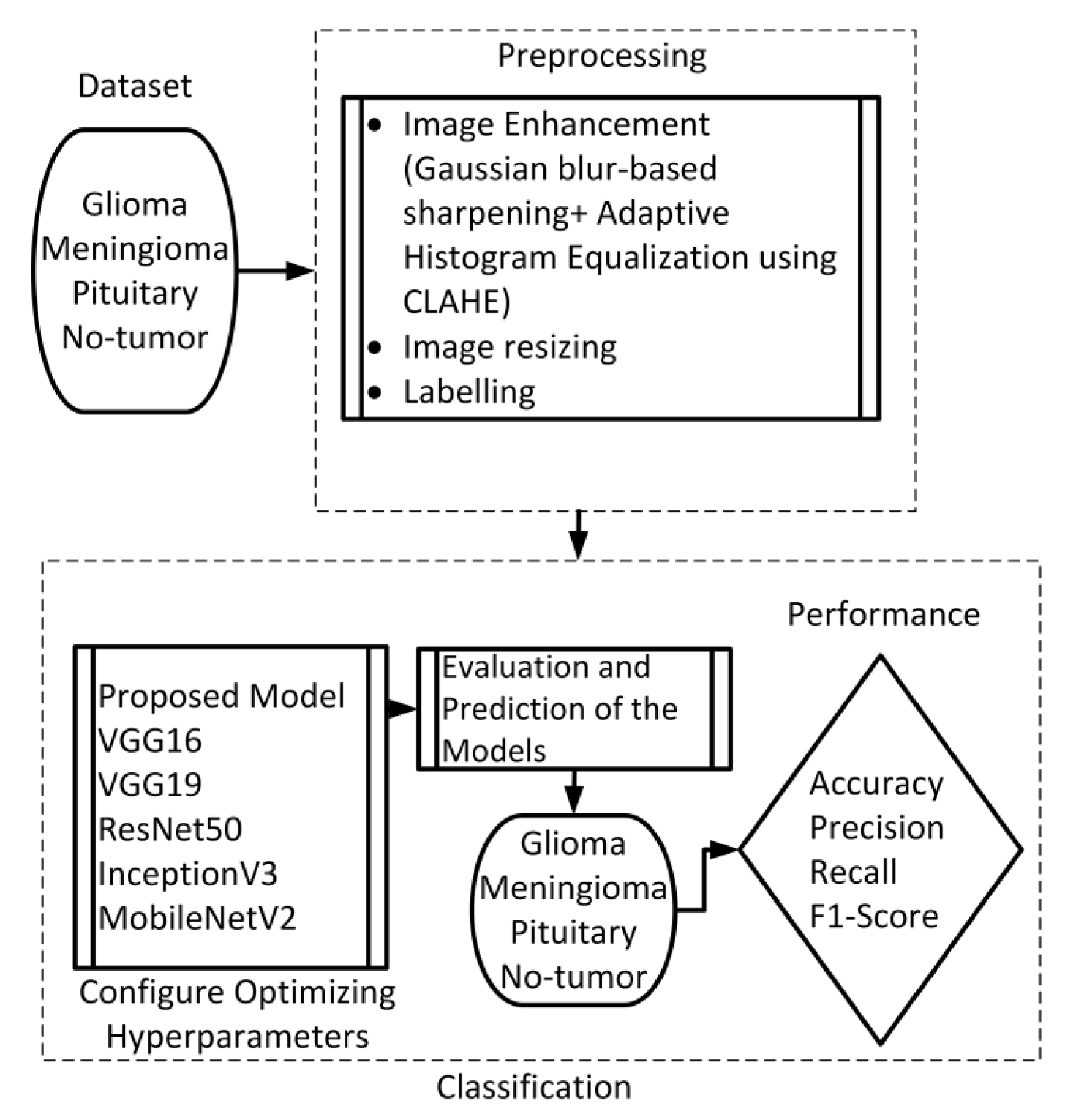
Figure 1. Flow chart of the suggested scheme.

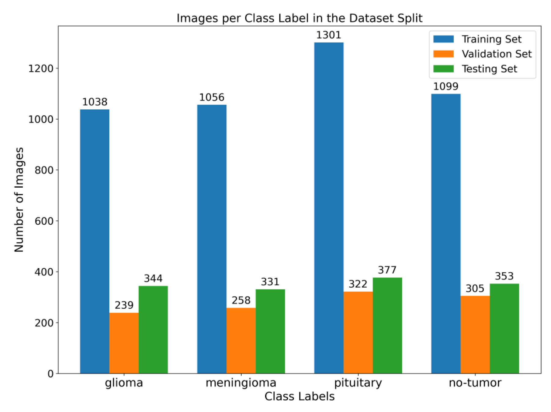
Figure 2. Illustration of the distribution of images among various class labels throughout the training, validation, and testing dataset splits. The bar graph displays the distribution of images across different classes, with the training set at 64%, the validation set at 16%, and the testing set at 20%.

This study employed a publicly accessible MRI dataset Msoud [45], obtained from the Kaggle repository. This dataset combines three publicly accessible datasets, including Figshare [46], SARTAJ [47], and BR35H [48]. It consists of 7023 MRIs of the human brain provided in grayscale and jpg format. The dataset includes primary types of brain tumors, namely glioma, meningioma, pituitary tumors, and images without tumors.

3.1. Preprocessing

We implemented a preprocessing framework to improve image quality by integrating sharpening and Contrast-Limited Adaptive Histogram Equalization (CLAHE) approaches. The process of sharpening commenced by implementing a Gaussian blur through the utilization of a specific technique. The utilization of a 5 × 5 kernel was suitable in the process of attenuating high-frequency noise. The resultant enhanced image was determined using the formula:

In order to ensure accordance with the specifications of the subsequent deep learning framework, the enhanced grayscale image was transformed into the RGB color space [49,50]. Figure 3 illustrates the several stages of enhancing picture quality, from the initial image to the CLAHE-enhanced image. This depiction showcases the effectiveness of our preprocessing method and its notable impact on improving the overall quality of the image.

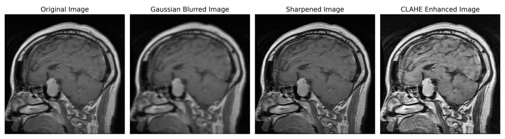
Figure 3. Sequential image improvement as part of the preprocessing framework. The stages progress from the unaltered original image through Gaussian blurring for noise suppression, sharpening the emphasized edge definition to the final enhancement using CLAHE.

3.2. Proposed Architecture

Figure 4 depicts the proposed model, which acquires MRI data with input dimensions of 224 × 224 and reveals its operational characteristics. The model consists of multiple server blocks. A convolutional layer [51] was employed in the initial stage, consisting of 16 filters. Each filter was employed with a kernel size of 3 × 3 and a stride size of 1 × 1. A normalizing layer [52] and a 2D (two-dimensional) max pooling layer with a size of 2 × 2 were employed to maximize the information among the intermediate layer’s output. Similarly, we integrated additional convolutional layers into the model, utilizing 32, 64, 128, and 256 filter sizes. Each filter utilized in this study had a kernel size of 3 × 3 and a stride size of 1 × 1, and the same and valid padding was suitable for the experiment. As illustrated in Figure 4, skip connections were employed within each block to facilitate the information flow by concatenating the outputs of specific convolutional layers. Subsequently, a dense layer of 512 neurons was employed, accompanied by global average pooling and activation through the rectified linear unit (ReLU) function.

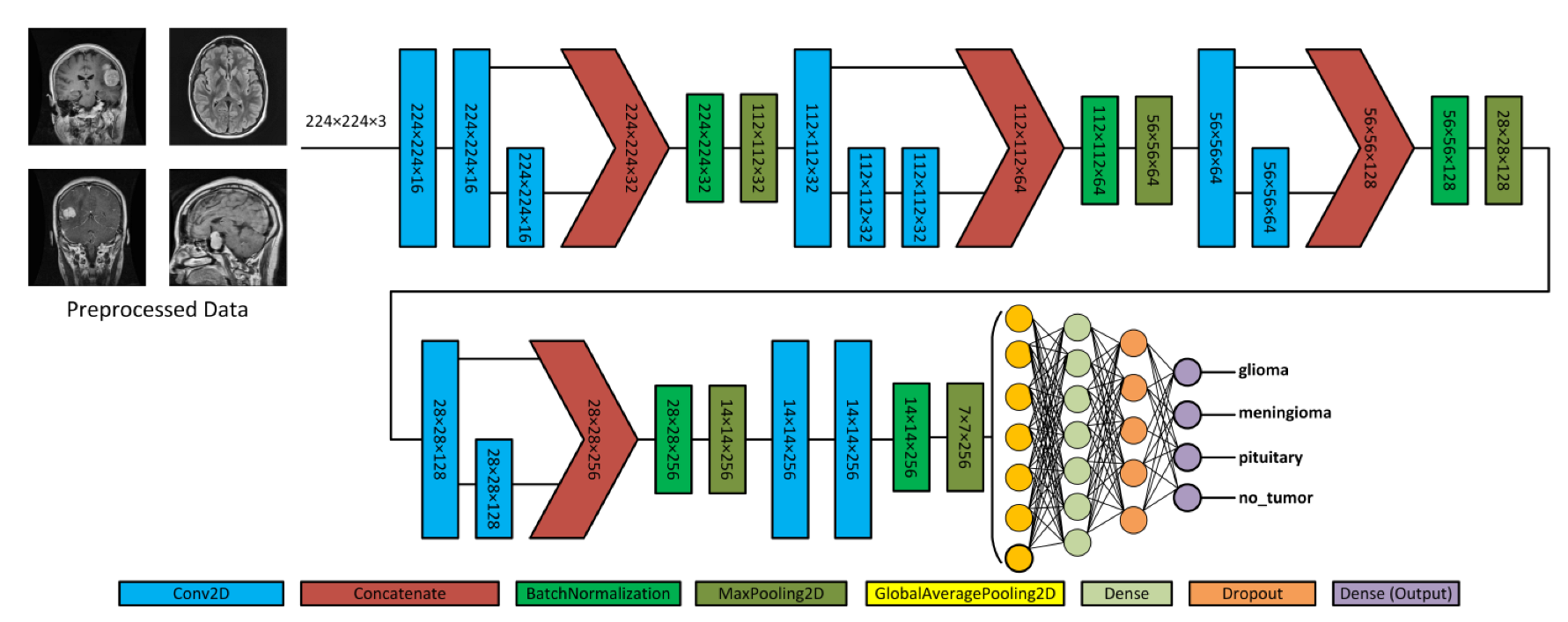
Figure 4. Illustration of the proposed architecture and various forms of brain tumors.

To mitigate the issue of overfitting, the dense layer was subjected to regulation using L1 (10⁻⁵) and L2 (10⁻⁴) regularization techniques [53]. During the training process, the neurons within a dropout layer [54] were randomly deactivated at a rate of 0.5% to enhance regularization implementation further. Finally, the output layer employed the softmax algorithm [51] to compute the probability score for each class and classify whether the input image exhibited a glioma, meningioma, pituitary, or no tumor. In addition, the model employed the Adam optimizer [55,56], categorical cross-entropy for loss functions, and the ReduceLROnPlateau callback to optimize the learning rate [57]. The model was trained with a batch size of 8 for 30 epochs.

Convolutional neural networks are widely used for image classification tasks. In the proposed model, 2D convolution involved applying a kernel to the input data to extract features. The convolution operation captures spatial dependencies and hierarchies within the data. The convolution operation in a 2D CNN can be mathematically defined as follows:

3.3. Pre-Trained Model

Pre-trained neural networks are ML models that have undergone training on extensive datasets like ImageNet, consisting of various images belonging to various classes. Pre-trained models have proven highly advantageous in various tasks, including image classification and object detection. Pre-trained models are employed because of their ability to graph data patterns, allowing them to be used as a starting point for new tasks without having to start the training process from scratch. This investigation included five pre-trained models, namely VGG16, ResNet50, MobileNetV2, InceptionV3, and VGG19.

4. Experimental Results

This study employed the proposed model to categorize a substantial MRI dataset comprising 7023 images. The dataset encompassed glioma, meningioma, pituitary cases, and cases with no tumor. Initially, a preprocessing stage was incorporated to enhance the feature extraction. In this stage, image enhancement techniques with Gaussian blur and CLAHE were applied to improve the quality of the images. The dataset was divided into subsets, namely training, validation, and testing. The dataset was trained using the Adam optimizer and subsequently assessed through a fivefold cross-validation method. Algorithm 1 presents the procedure for the training and evaluation process.

The learning rates were optimized using the ReduceLROnPlateau callbacks, and a batch size of 8 was utilized. Figure 6 presents the average accuracy and losses of the model proposed in this study. During the initial stage of training, the graphs display fluctuations, which can be attributed to the utilization of the ReduceLROnPlateau callback. The primary objective of this callback is to dynamically modify the learning rate of the optimizer during the training process, specifically when the loss function reaches a plateau. After completing 12 epochs, the optimizer demonstrates a gradual convergence toward an optimal configuration of weights, resulting in diminished fluctuations observed in the accuracy and loss curves.

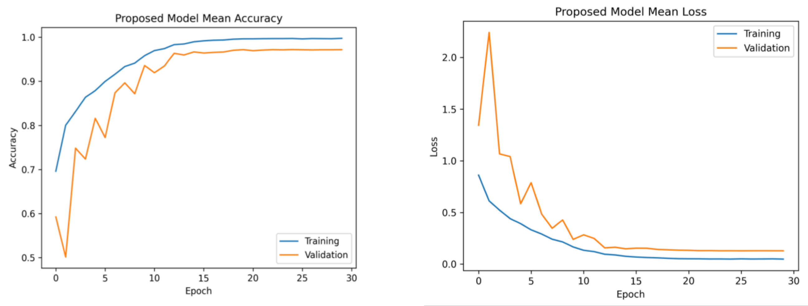
Figure 6. Mean accuracy and losses of the proposed model during 5-fold cross-validation. (Left): mean accuracy progression across training folds. (Right): corresponding mean loss trend. This demonstrates consistent accuracy improvement and decreasing loss, highlighting effective model training.

Furthermore, the platform utilized several libraries, such as Numpy, Pandas, Matplotlib, Sklearn, Keras, and TensorFlow, to enhance the efficiency of data processing and model development. The computation was performed on an Intel Core i7-7800 CPU operating at a clock speed of 3.5 GHz. The model training and tuning were managed using an NVIDIA GeForce GTX 1080 Ti GPU. The selection of Python 3.7 as the primary programming language for this study was based on its comprehensive set of tools for data manipulation, analysis, and visualization. The platform successfully preserved the data employed in this study due to its substantial RAM capacity of 32 GB.

Model Evaluation Matrices

The suggested framework was subjected to a thorough evaluation, which involved an analysis of its precision, recall, F1-score, and accuracy. Precision evaluates the model’s ability to minimize the misclassification of negative examples as positive, and the term “is derived from” refers to the calculation of a specific metric, which is obtained by dividing the number of true positives by the sum of true positives and false positives. However, it is important to note that recall is a metric that measures the model’s capacity to classify the appropriate tumor type accurately. This is calculated by dividing the number of true positives by the sum of true positives and false negatives. The F1-score is a metric used in evaluation that quantifies the balance between precision and recall. It is calculated as the harmonic mean of precision and recall, obtained by multiplying precision and recall and dividing the result by their sum, multiplied by two. In the context of classification models, accuracy measures the model’s overall performance by quantifying the proportion of correct classifications. It is calculated by dividing the number of accurate predictions by the total number of predictions made. Equations (13)–(16) indicate the mathematical representations of precision, recall, F1-score, and accuracy [67].

The evaluation results, including the average precision, recall, F1-score, and accuracy for both the proposed and pre-trained models, are presented in . The suggested framework demonstrated a notable accuracy rate of 97.84%. Moreover, it achieved precision and recall values of 97.85% and an F1-score of 97.90%. On the contrary, the InceptionV3 model exhibited the lowest performance, achieving an accuracy of 88.15%, a precision rate of 87.70%, a recall rate of 87.89%, and an F1-score rate of 87.60%. The observed variation in the performance of InceptionV3 can be ascribed to its utilization of multiple and parallel modules, which may not be well suited for the specific characteristics of this dataset, as supported by our research findings. The pre-trained models VGG16, ResNet50, and VGG19 exhibited superior performance compared to MobileNetV2. Furthermore, the pre-trained models employed the standard input dimensions, including VGG16, VGG19, ResNet50, and MobileNetV2 with dimensions of 224 × 224 and InceptionV3 with dimensions of 299 × 229. In order to preserve the pre-existing weights, the layers of the base model were designated as non-trainable.

The utilization of the confusion matrix is a fundamental assessment instrument for classification models [68]. The proposed network demonstrated robust capabilities in accurately classifying various types of brain tumors, effectively identifying each type during the examination. Figure 7 presents a visual representation of the results obtained from the testing data, enabling a comparison between the proposed and pre-trained models. The comparison reveals that the proposed model outperformed the pre-trained models in performance. The proposed model demonstrated high accuracy in predicting glioma, achieving 97%, and meningioma, achieving a 96% accuracy rate. Additionally, it achieved a 99% accuracy rate in predicting pituitary and no-tumor cases. These results surpass the performance of pre-trained models. However, it is crucial to emphasize that the efficacy of treatment for glioma and meningioma in this study did not achieve comparable levels of success. This finding underscores the necessity for additional research and investigation in subsequent studies.

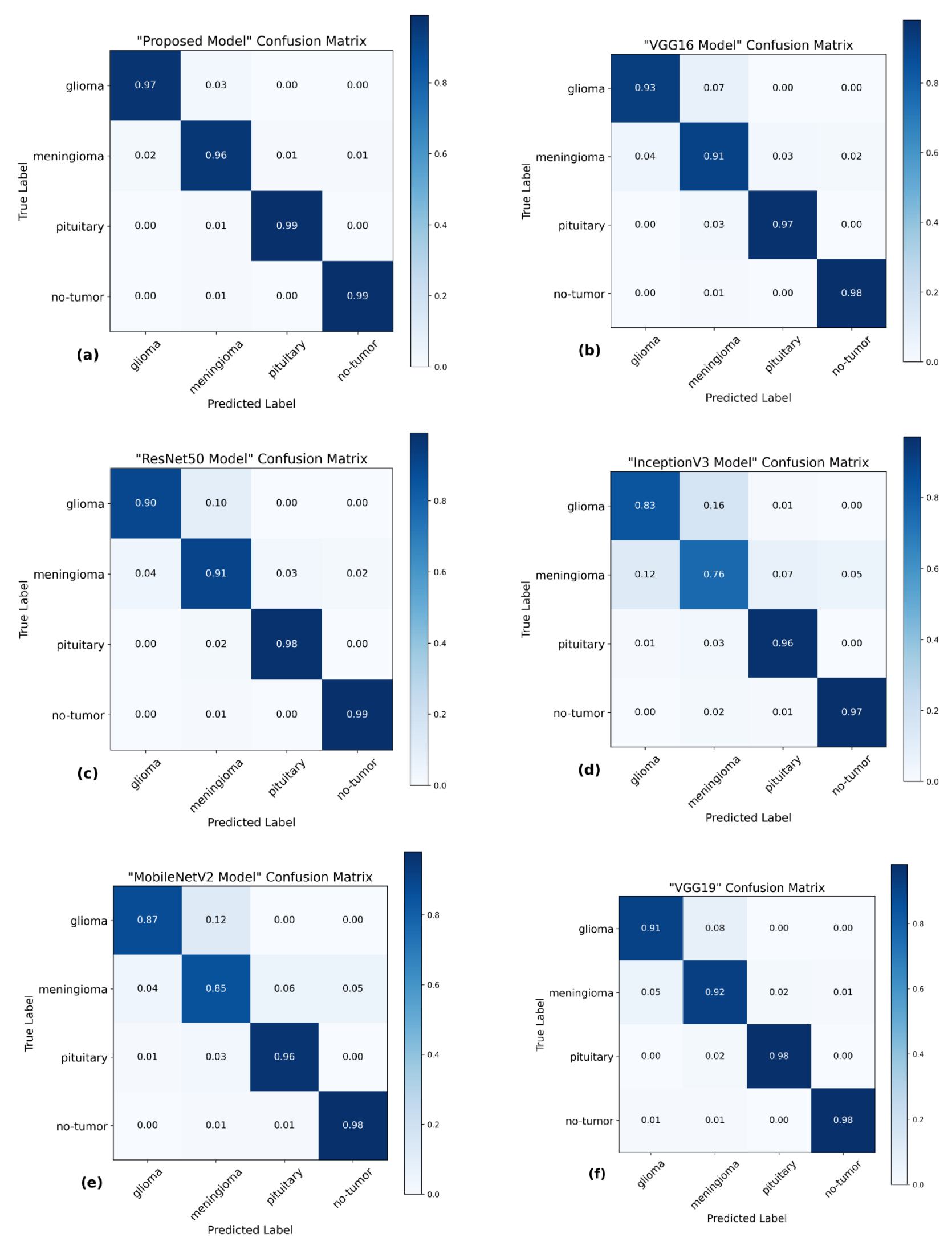
Figure 7. Confusion matrices of several models using the testing data. (a) The proposed model has a high level of accuracy, achieving a score of 97.84%. (b) VGG16 model achieved a classification accuracy of 95.00%. (c) ResNet50 model achieved an accuracy of 94.75%. (d) The accuracy of InceptionV3 is 88.15%. (e) MobileNetV2 model achieved a classification accuracy of 91.73%. (f) VGG19 model achieved a classification accuracy of 94.83%.

Furthermore, the Receiver Operating Characteristics (ROC) curve is a visual representation of the performance of a classification model across different classification thresholds [69]. The True Positive Rate (TPR) and False Positive Rate (FPR) are graphically represented. The ROC curve illustrates the balance between correctly identifying positive and incorrectly classifying negative instances as positive at all classification thresholds on the testing set. The ROC curve provides insights into the model’s ability to differentiate between different thresholds effectively.

The present investigation demonstrates the proposed framework’s superior diagnostic efficacy compared to pre-trained designs. The findings of this study provide evidence supporting the suggested model’s higher diagnostic accuracy compared to state-of-the-art methodologies. When comparing the performance of the VGG16 architecture, it was observed that it achieved scores of 0.95 for glioma, 0.93 for meningioma, 0.97 for pituitary, and 0.98 for the no-tumor category. The ResNet50 architecture achieved classification scores of 0.92, 0.93, 0.97, and 0.98 for the glioma, meningioma, pituitary, and no-tumor classes, respectively. The InceptionV3 model yielded predictive scores of 0.84 for glioma, 0.81 for meningioma, 0.96 for pituitary, and 0.97 for the no-tumor category. The MobileNetV2 design achieved scores of 0.90, 0.86, 0.97, and 0.98 for the glioma, meningioma, pituitary, and no-tumor categories, respectively. Additionally, the VGG19 architecture demonstrated classification scores of 0.92 for glioma, 0.93 for meningioma, 0.98 for the pituitary, and 0.98 for the no-tumor category.

The model under consideration demonstrates notable performance regarding ROC scores. The achieved classification accuracies are as follows: 0.98 for glioma, 0.97 for meningioma, 0.99 for pituitary, and a flawless accuracy of 1.00 for the no-tumor category. The robust performance of the model is supported by a collective ROC score of 98.50%, as depicted in Figure 8, compared to pre-trained models.

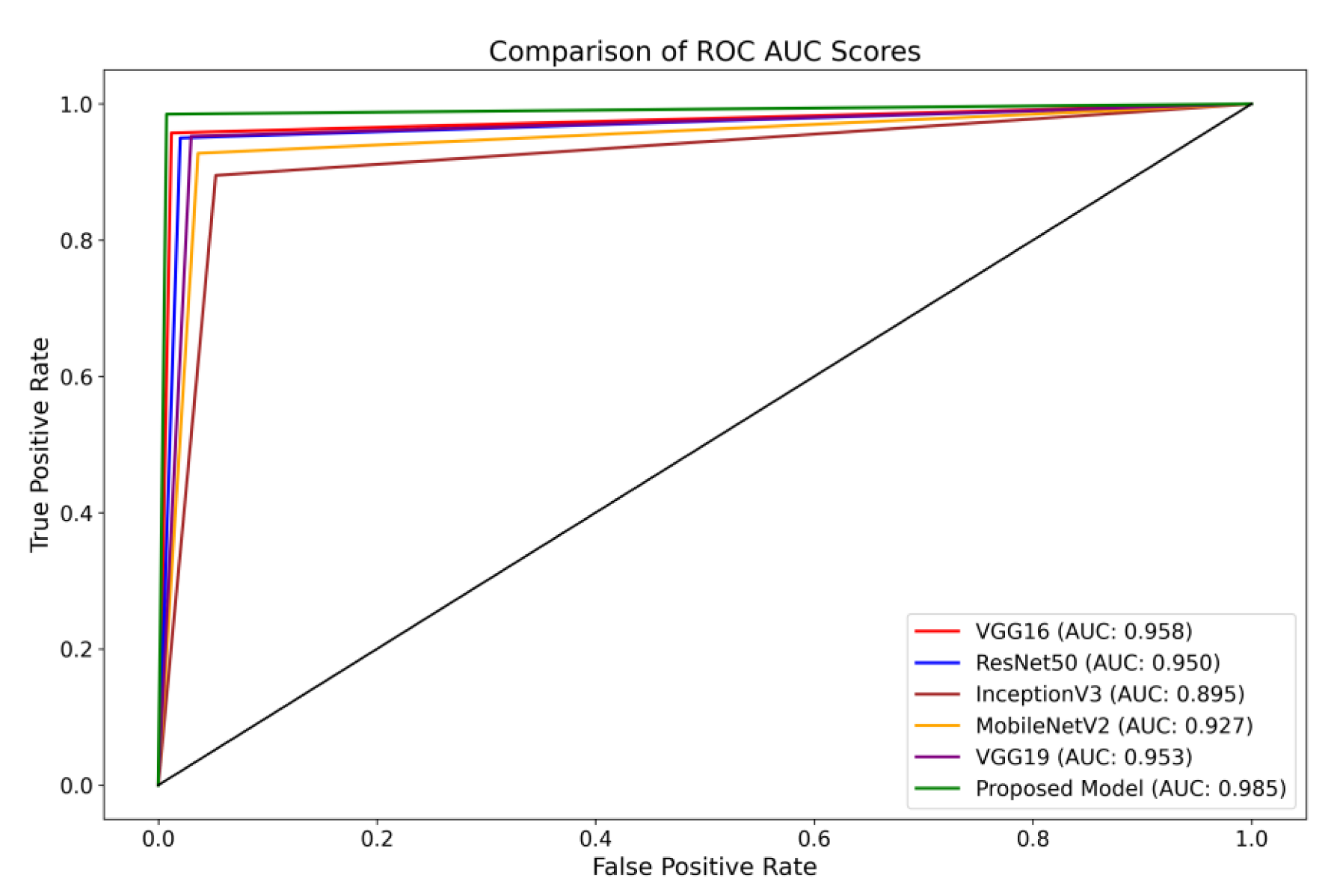
Figure 8. Illustration of a comprehensive visual representation that compares the proposed model’s overall ROC score with other pre-trained models.

5. Discussion

This investigation introduces a novel methodology for categorizing the Msoud dataset, which consists of a varied assortment of 7023 brain images. The efficacy of the proposed system is demonstrated by its capacity to attain highly precise prediction outcomes, surpassing prior research endeavors with comparable aims. Moreover, this study proposes a method that does not rely on segmenting brain tumor images for classification purposes. The primary advantage of our approach resides in its capacity to substantially diminish the requirement for manual procedures, such as feature extraction and tumor localization. These processes are not only time-intensive but also susceptible to inaccuracies. By employing various enhancement techniques, including sharpening with Gaussian blur and Contrast-Limited Adaptive Histogram Equalization (CLAHE), notable enhancements are achieved in the quality of the brain images. The enhancement process plays a crucial role in the refinement of edges and improving the overall image clarity, reducing the manual effort needed for feature extraction.

Furthermore, our proposed model incorporates distinctive concatenation concepts within the convolutional layers, demonstrating superior performance compared to alternative methods, as shown in . By incorporating these enhancement techniques, the proposed model has demonstrated exceptional performance, surpassing the existing state-of-the-art model in classifying brain tumors. The successful accomplishment is evidence of the proposed model’s resilience and capacity to apply to a wide range of brain image classification tasks, highlighting its potential for achieving precise and dependable results. Integrating decreased manual intervention, enhanced image quality, and the suggested model architecture renders our approach highly promising for practical implementations in classifying brain tumors.

The methodology of Gumaei et al. [25] introduced a combination of PCA, NGIST, and RELM. While this hybrid approach attempted to capture a comprehensive feature set, PCA might not always capture non-linear patterns inherent in brain images, potentially missing crucial tumor-specific details and resulting in less accuracy. The methodologies of Swati et al. [40] and Noreen et al. [34] relied on refining generic architectures, specifically state-of-the-art models. Such fine-tuning of deep architectures can be resource-intensive. The intricate process necessitates substantial computational resources and proves time-consuming, given the need to adjust many parameters in these extensive networks. Contrarily, our model is purposefully designed for brain tumor classification. It captures tumor-specific attributes efficiently without the excessive computational demands typically associated with deep architectures. As corroborated by , our method requires fewer parameters than the state of the art and delivers faster testing times.

Ghassemi et al. [32] ventured into the territory of Generative Adversarial Networks, leveraging CNN-based GANs. While GANs are adept at generating synthetic images, their direct application to classification might introduce synthetic nuances that deviate from real-world MRI variations, potentially affecting classification accuracy. Huang et al. [31] introduced the CNNBCN, a model rooted in randomly generated graph algorithms, achieving an accuracy of 95.49% and demonstrating advancements in neural network design. In contrast, our methodology performs superior classification on extensive tumor and no-tumor images.

Techniques like HDWT-HOG-Bagging and NLBP-αLBP-KNN, as presented by Fouad et al. [27] and Kaplan et al. [19], rely heavily on traditional feature extraction. While computationally intensive, such methods might still miss subtle details and patterns in the MRI scans, resulting in less accuracy. Ayadi et al. [28] employed DSURF-HOG combined with SVM for classification, a method that might overlook hierarchical and spatial patterns in MRI images, which deep learning models can capture more effectively.

Ekong et al. [41] introduced a Bayesian-CNN approach, and while Bayesian methods offer probabilistic insights, they might not always capture the intricate features of brain tumors. While the GAN-Softmax approach by Asiri et al.’s [42] model offers certain advancements, it is computationally more demanding. Moreover, the efficacy of methodologies such as HOG-XG Boost by Shilaskar et al. [43] and the SURF-KAZE technique by Almalki et al. [38] might be constrained, particularly in their ability to capture spatial and hierarchical MRI patterns—areas where contemporary deep learning models exhibit proficiency as proved in this study.

Limitations

The usefulness of the proposed methodology for extracting features has been proven by using a specific dataset obtained from MRI scans. In order to enhance the clarity of the images, various techniques for image enhancement were employed. Although these strategies can enhance visibility, it is crucial to acknowledge that, in specific circumstances, it may impact classification accuracy. Therefore, comprehensive evaluations are necessary to test the method’s suitability for different imaging modalities and clinical scenarios and its flexibility for image enhancements.

6. Conclusions

The present study introduced a novel approach to classify various categories of brain tumors, such as primary, meningioma, pituitary, and instances with no tumor. This is achieved by combining image enhancement techniques, namely, Gaussian-blur-based sharpening and Contrast-Limited Adaptive Histogram Equalization (CLAHE), with a proposed convolutional neural network. The findings of our study demonstrate a remarkable level of accuracy, specifically 97.84%, which was achieved through a diligent evaluation of the effectiveness of the suggested framework. The outcome of this study showcases the model’s robust capacity for generalization, rendering it a valuable and dependable tool within the medical field. The capacity of this method to facilitate expeditious and accurate decision making by medical professionals in the realm of brain tumor diagnosis is evident. To enhance patient care in the future, we intend to revolutionize medical imaging methods. This will be accomplished by creating real-time brain tumor detection systems and establishing three-dimensional networks to analyze other medical images.

References

1. Khazaei, Z.; Goodarzi, E.; Borhaninejad, V.; Iranmanesh, F.; Mirshekarpour, H.; Mirzaei, B.; Naemi, H.; Bechashk, S.M.; Darvishi, I.; Ershad Sarabi, R.; et al. The association between incidence and mortality of brain cancer and human development index (HDI): An ecological study. BMC Public Health 2020, 20, 1696. [Google Scholar] [CrossRef]
2. GLOBOCAN. The Global Cancer Observatory—All Cancers. Int. Agency Res. Cancer—WHO 2020, 419, 199–200. Available online: https://gco.iarc.fr/today/home (accessed on 12 February 2023).
3. Johns Hopkins Medicine. Gliomas. Available online: https://www.hopkinsmedicine.org/health/conditions-and-diseases/gliomas (accessed on 12 February 2023).
4. Mayo Clinic. Pituitary Tumors—Symptoms and Causes. Available online: https://www.mayoclinic.org/diseases-conditions/pituitary-tumors/symptoms-causes/syc-20350548 (accessed on 12 February 2023).
5. Johns Hopkins Medicine. Meningioma. Available online: https://www.hopkinsmedicine.org/health/conditions-and-diseases/meningioma (accessed on 12 February 2023).
6. Merck Manuals Consumer Version. Overview of Brain Tumors—Brain, Spinal Cord, and Nerve Disorders. Available online: https://www.merckmanuals.com/home/brain,-spinal-cord,-and-nerve-disorders/tumors-of-the-nervous-system/overview-of-brain-tumors (accessed on 17 May 2022).
7. American Brain Tumor Association. American Brain Tumor Association Mood Swings and Cognitive Changes. 2014. Available online: https://web.archive.org/web/20160802203516/http://www.abta.org/brain-tumor-information/symptoms/mood-swings.html (accessed on 11 December 2022).
8. Tiwari, A.; Srivastava, S.; Pant, M. Brain tumor segmentation and classification from magnetic resonance images: Review of selected methods from 2014 to 2019. Pattern Recognit. Lett. 2020, 131, 244–260. [Google Scholar] [CrossRef]
9. Iwendi, C.; Khan, S.; Anajemba, J.H.; Mittal, M.; Alenezi, M.; Alazab, M. The use of ensemble models for multiple class and binary class classification for improving intrusion detection systems. Sensors 2020, 20, 2559. [Google Scholar] [CrossRef] [PubMed]
10. Ahmad, S.; Ullah, T.; Ahmad, I.; Al-Sharabi, A.; Ullah, K.; Khan, R.A.; Rasheed, S.; Ullah, I.; Uddin, M.N.; Ali, M.S. A Novel Hybrid Deep Learning Model for Metastatic Cancer Detection. Comput. Intell. Neurosci. 2022, 2022, 8141530. [Google Scholar] [CrossRef] [PubMed]
11. Zhuang, Y.; Chen, S.; Jiang, N.; Hu, H. An Effective WSSENet-Based Similarity Retrieval Method of Large Lung CT Image Databases. KSII Trans. Internet Inf. Syst. 2022, 16, 2359–2376. [Google Scholar] [CrossRef]
12. Li, C.; Lin, L.; Zhang, L.; Xu, R.; Chen, X.; Ji, J.; Li, Y. Long noncoding RNA p21 enhances autophagy to alleviate endothelial progenitor cells damage and promote endothelial repair in hypertension through SESN2/AMPK/TSC2 pathway. Pharmacol. Res. 2021, 173, 105920. [Google Scholar] [CrossRef]
13. Deng, X.; Liu, E.; Li, S.; Duan, Y.; Xu, M. Interpretable Multi-Modal Image Registration Network Based on Disentangled Convolutional Sparse Coding. IEEE Trans. Image Process. 2023, 32, 1078–1091. [Google Scholar] [CrossRef]
14. Zhang, K.; Yang, Y.; Ge, H.; Wang, J.; Lei, X.; Chen, X.; Wan, F.; Feng, H.; Tan, L. Neurogenesis and Proliferation of Neural Stem/Progenitor Cells Conferred by Artesunate via FOXO3a/p27Kip1 Axis in Mouse Stroke Model. Mol. Neurobiol. 2022, 59, 4718–4729. [Google Scholar] [CrossRef]
15. Wang, F.; Wang, H.; Zhou, X.; Fu, R. A Driving Fatigue Feature Detection Method Based on Multifractal Theory. IEEE Sens. J. 2022, 22, 19046–19059. [Google Scholar] [CrossRef]
16. Gao, Z.; Pan, X.; Shao, J.; Jiang, X.; Su, Z.; Jin, K.; Ye, J. Automatic interpretation and clinical evaluation for fundus fluorescein angiography images of diabetic retinopathy patients by deep learning. Br. J. Ophthalmol. 2022, 1–7. [Google Scholar] [CrossRef] [PubMed]
17. Xu, H.; Van Der Jeught, K.; Zhou, Z.; Zhang, L.; Yu, T.; Sun, Y.; Li, Y.; Wan, C.; So, K.M.; Liu, D.; et al. Atractylenolide I enhances responsiveness to immune checkpoint blockade therapy by activating tumor antigen presentation. J. Clin. Investig. 2021, 131, e146832. [Google Scholar] [CrossRef] [PubMed]
18. Ao, J.; Shao, X.; Liu, Z.; Liu, Q.; Xia, J.; Shi, Y.; Qi, L.; Pan, J.; Ji, M. Stimulated Raman Scattering Microscopy Enables Gleason Scoring of Prostate Core Needle Biopsy by a Convolutional Neural Network. Cancer Res. 2023, 83, 641–651. [Google Scholar] [CrossRef] [PubMed]
19. Kaplan, K.; Kaya, Y.; Kuncan, M.; Ertunç, H.M. Brain tumor classification using modified local binary patterns (LBP) feature extraction methods. Med. Hypotheses 2020, 139, 109696. [Google Scholar] [CrossRef]
20. Rathi, V.G.P.; Palani, S. Brain Tumor Detection and Classification Using Deep Learning Classifier on MRI Images. Res. J. Appl. Sci. Eng. Technol. 2015, 10, 177–187. [Google Scholar] [CrossRef]
21. Cheng, J.; Huang, W.; Cao, S.; Yang, R.; Yang, W.; Yun, Z.; Wang, Z.; Feng, Q. Enhanced Performance of Brain Tumor Classification via Tumor Region Augmentation and Partition. PLoS ONE 2015, 10, e0140381. [Google Scholar] [CrossRef]
22. McBee, M.P.; Awan, O.A.; Colucci, A.T.; Ghobadi, C.W.; Kadom, N.; Kansagra, A.P.; Tridandapani, S.; Auffermann, W.F. Deep Learning in Radiology. Acad. Radiol. 2018, 25, 1472–1480. [Google Scholar] [CrossRef]
23. Lu, S.; Yang, J.; Yang, B.; Yin, Z.; Liu, M.; Yin, L.; Zheng, W. Analysis and Design of Surgical Instrument Localization Algorithm. Comput. Model. Eng. Sci. 2022, 137, 669–685. [Google Scholar] [CrossRef]
24. Afshar, P.; Plataniotis, K.N.; Mohammadi, A. Capsule Networks for Brain Tumor Classification Based on MRI Images and Coarse Tumor Boundaries. In Proceedings of the ICASSP 2019—2019 IEEE International Conference on Acoustics, Speech and Signal Processing (ICASSP), Brighton, UK, 12–17 May 2019; pp. 1368–1372. [Google Scholar] [CrossRef]
25. Gumaei, A.; Hassan, M.M.; Hassan, M.R.; Alelaiwi, A.; Fortino, G. A Hybrid Feature Extraction Method with Regularized Extreme Learning Machine for Brain Tumor Classification. IEEE Access 2019, 7, 36266–36273. [Google Scholar] [CrossRef]
26. Rezaei, K.; Agahi, H.; Mahmoodzadeh, A. A Weighted Voting Classifiers Ensemble for the Brain Tumors Classification in MR Images. IETE J. Res. 2020, 68, 3829–3842. [Google Scholar] [CrossRef]
27. Fouad, A.; Moftah, H.M.; Hefny, H.A. Brain diagnoses detection using whale optimization algorithm based on ensemble learning classifier. Int. J. Intell. Eng. Syst. 2020, 13, 40–51. [Google Scholar] [CrossRef]
28. Ayadi, W.; Charfi, I.; Elhamzi, W.; Atri, M. Brain tumor classification based on hybrid approach. Vis. Comput. 2020, 38, 107–117. [Google Scholar] [CrossRef]
29. Srujan, K.S.; Shivakumar, S.; Sitnur, K.; Garde, O.; Pk, P. Brain Tumor Segmentation and Classification using CNN model. Int. Res. J. Eng. Technol. 2020, 7, 4077–4080. [Google Scholar]
30. Tejaswini, G.P.; Sreelakshmi, K. Brain Tumour Detection using Deep Neural Network. Wutan Huatan Jisuan Jishu 2020, XVI, 27–40. [Google Scholar]
31. Huang, Z.; Du, X.; Chen, L.; Li, Y.; Liu, M.; Chou, Y.; Jin, L. Convolutional Neural Network Based on Complex Networks for Brain Tumor Image Classification with a Modified Activation Function. IEEE Access 2020, 8, 89281–89290. [Google Scholar] [CrossRef]
32. Ghassemi, N.; Shoeibi, A.; Rouhani, M. Deep neural network with generative adversarial networks pre-training for brain tumor classification based on MR images. Biomed. Signal Process. Control 2020, 57, 101678. [Google Scholar] [CrossRef]
33. Deepak, S.; Ameer, P.M. Automated Categorization of Brain Tumor from MRI Using CNN features and SVM. J. Ambient Intell. Humaniz. Comput. 2020, 12, 8357–8369. [Google Scholar] [CrossRef]
34. Noreen, N.; Palaniappan, S.; Qayyum, A.; Ahmad, I.; Alassafi, M.O. Brain Tumor Classification Based on Fine-Tuned Models and the Ensemble Method. Comput. Mater. Contin. 2021, 67, 3967–3982. [Google Scholar] [CrossRef]
35. Shaik, N.S.; Cherukuri, T.K. Multi-level attention network: Application to brain tumor classification. Signal Image Video Process. 2022, 16, 817–824. [Google Scholar] [CrossRef]
36. Ahmad, B.; Sun, J.; You, Q.; Palade, V.; Mao, Z. Brain Tumor Classification Using a Combination of Variational Autoencoders and Generative Adversarial Networks. Biomedicines 2022, 10, 223. [Google Scholar] [CrossRef]
37. Alanazi, M.F.; Ali, M.U.; Hussain, S.J.; Zafar, A.; Mohatram, M.; Irfan, M.; Alruwaili, R.; Alruwaili, M.; Ali, N.H.; Albarrak, A.M. Brain Tumor/Mass Classification Framework Using Magnetic-Resonance-Imaging-Based Isolated and Developed Transfer Deep-Learning Model. Sensors 2022, 22, 372. [Google Scholar] [CrossRef] [PubMed]
38. Almalki, Y.E.; Ali, M.U.; Ahmed, W.; Kallu, K.D.; Zafar, A.; Alduraibi, S.K.; Irfan, M.; Basha, M.A.A.; Alshamrani, H.A.; Alduraibi, A.K. Robust Gaussian and Nonlinear Hybrid Invariant Clustered Features Aided Approach for Speeded Brain Tumor Diagnosis. Life 2022, 12, 1084. [Google Scholar] [CrossRef] [PubMed]
39. Kavin Kumar, K.; Dinesh, P.M.; Rayavel, P.; Vijayaraja, L.; Dhanasekar, R.; Kesavan, R.; Raju, K.; Khan, A.A.; Wechtaisong, C.; Haq, M.A.; et al. Brain Tumor Identification Using Data Augmentation and Transfer Learning Approach. Comput. Syst. Sci. Eng. 2023, 46, 1845–1861. [Google Scholar] [CrossRef]
40. Swati, Z.N.K.; Zhao, Q.; Kabir, M.; Ali, F.; Ali, Z.; Ahmed, S.; Lu, J. Brain tumor classification for MR images using transfer learning and fine-tuning. Comput. Med. Imaging Graph. 2019, 75, 34–46. [Google Scholar] [CrossRef] [PubMed]
41. Ekong, F.; Yu, Y.; Patamia, R.A.; Feng, X.; Tang, Q.; Mazumder, P.; Cai, J. Bayesian Depth-Wise Convolutional Neural Network Design for Brain Tumor MRI Classification. Diagnostics 2022, 12, 1657. [Google Scholar] [CrossRef]
42. Asiri, A.A.; Shaf, A.; Ali, T.; Aamir, M.; Usman, A.; Irfan, M.; Alshamrani, H.A.; Mehdar, K.M.; Alshehri, O.M.; Alqhtani, S.M. Multi-Level Deep Generative Adversarial Networks for Brain Tumor Classification on Magnetic Resonance Images. Intell. Autom. Soft Comput. 2023, 36, 127–143. [Google Scholar] [CrossRef]
43. Shilaskar, S.; Mahajan, T.; Bhatlawande, S.; Chaudhari, S.; Mahajan, R.; Junnare, K. Machine Learning Based Brain Tumor Detection and Classification using HOG Feature Descriptor. In Proceedings of the International Conference on Sustainable Computing and Smart Systems, ICSCSS, Coimbatore, India, 14–16 June 2023; pp. 67–75. [Google Scholar]
44. Yadav, S. Analysis of k-fold cross-validation over hold-out validation on colossal datasets for quality classification. In Proceedings of the 2016 IEEE 6th International Conference on Advanced Computing (IACC), Bhimavaram, India, 27–28 February 2016. [Google Scholar] [CrossRef]
45. Nickparvar, M.; Brain_Tumor_MRI Dataset. Kaggle. Dataset. 2021. Available online: https://www.kaggle.com/datasets/masoudnickparvar/brain-tumor-mri-dataset (accessed on 10 May 2023).
46. Cheng, J.; Brain Tumor Dataset. Figshare. 2017. Available online: https://figshare.com/articles/dataset/brain_tumor_dataset/1512427 (accessed on 10 May 2023).
47. Kaggle. Brain Tumor Classification (MRI). Available online: https://www.kaggle.com/datasets/sartajbhuvaji/brain-tumor-classification-mri (accessed on 10 July 2023).
48. Hamada, A. Br35H: Brain Tumor Detection. 2020. Available online: https://www.kaggle.com/datasets/ahmedhamada0/brain-tumor-detection (accessed on 10 May 2023).
49. Wang, W.; Chen, Z.; Yuan, X. Simple low-light image enhancement based on Weber–Fechner law in logarithmic space. Signal Process. Image Commun. 2022, 106, 116742. [Google Scholar] [CrossRef]
50. Wang, Y.; Su, Y.; Li, W.; Xiao, J.; Li, X.; Liu, A.A. Dual-path Rare Content Enhancement Network for Image and Text Matching. IEEE Trans. Circuits Syst. Video Technol. 2023; Early Access. [Google Scholar] [CrossRef]
51. Goodfellow, I.; Bengio, Y.; Courville, A. Deep Learning; MIT Press: Cambridge, MA, USA, 2016; pp. 1–10. Available online: https://www.deeplearningbook.org (accessed on 10 May 2023).
52. Ioffe, S.; Szegedy, C. Batch normalization: Accelerating deep network training by reducing internal covariate shift. In Proceedings of the 32nd International Conference on Machine Learning, Lille, France, 6–11 July 2015; Volume 1, pp. 448–456. [Google Scholar]
53. Alzubaidi, L.; Zhang, J.; Humaidi, A.J.; Al-Dujaili, A.; Duan, Y.; Al-Shamma, O.; Santamaría, J.; Fadhel, M.A.; Al-Amidie, M.; Farhan, L. Review of Deep Learning: Concepts, CNN Architectures, Challenges, Applications, Future Directions; Springer International Publishing: Cham, Switzerland, 2021; Volume 8, ISBN 4053702100444. [Google Scholar]
54. Bin Tufail, A.; Ullah, I.; Rehman, A.U.; Khan, R.A.; Khan, M.A.; Ma, Y.K.; Hussain Khokhar, N.; Sadiq, M.T.; Khan, R.; Shafiq, M.; et al. On Disharmony in Batch Normalization and Dropout Methods for Early Categorization of Alzheimer’s Disease. Sustainability 2022, 14, 14695. [Google Scholar] [CrossRef]
55. Kingma, D.P.; Ba, J. Adam: A Method for Stochastic Optimization. In Proceedings of the 3rd International Conference on Learning Representations, San Diego, CA, USA, 7–9 May 2015; Conference Track Proceedings. 2014; pp. 1–15. [Google Scholar]
56. Robbins, H.; Monro, S. A Stochastic Approximation Method. Ann. Math. Stat. 1951, 22, 400–407. [Google Scholar] [CrossRef]
57. Rasheed, Z.; Ma, Y.-K.; Ullah, I.; Al Shloul, T.; Bin Tufail, A.; Ghadi, Y.Y.; Khan, M.Z.; Mohamed, H.G. Automated Classification of Brain Tumors from Magnetic Resonance Imaging Using Deep Learning. Brain Sci. 2023, 13, 602. [Google Scholar] [CrossRef]
58. Nair, V.; Hinton, G.E. Rectified linear units improve Restricted Boltzmann machines. In Proceedings of the 27th International Conference on Machine Learning, Haifa, Israel, 21–24 June 2010; Association for Computing Machinery: New York, NY, USA, 2010. [Google Scholar]
59. Srivastava, N.; Hinton, G.; Krizhevsky, A.; Sutskever, I.; Salakhutdinov, R. Dropout: A Simple Way to Prevent Neural Networks from Overfitting. J. Mach. Learn. Res. 2014, 15, 1929–1958. [Google Scholar]
60. Moradi, R.; Berangi, R.; Minaei, B. A Survey of Regularization Strategies for Deep Models. Artif. Intell. Rev. 2020, 53, 3947–3986. [Google Scholar] [CrossRef]
61. ReduceLROnPlateau. Available online: https://keras.io/api/callbacks/reduce_lr_on_plateau/ (accessed on 24 May 2023).
62. Simonyan, K.; Zisserman, A. Very deep convolutional networks for large-scale image recognition. In Proceedings of the 3rd International Conference on Learning Representations, San Diego, CA, USA, 7–9 May 2015. Conference Track Proceedings. [Google Scholar]
63. Glorot, X.; Bengio, Y. Understanding the difficulty of training deep feedforward neural networks. J. Mach. Learn. Res. 2010, 9, 249–256. [Google Scholar]
64. He, K.; Zhang, X.; Ren, S.; Sun, J. Deep residual learning for image recognition. In Proceedings of the IEEE Conference on Computer Vision and Pattern Recognition (CVPR), Las Vegas, NV, USA, 27–30 June 2016; Volume 2016, pp. 770–778. [Google Scholar] [CrossRef]
65. Sandler, M.; Howard, A.; Zhu, M.; Zhmoginov, A.; Chen, L.C. MobileNetV2: Inverted Residuals and Linear Bottlenecks. In Proceedings of the 2018 IEEE Conference on Computer Vision and Pattern Recognition (CVPR), Salt Lake City, UT, USA, 18–23 June 2018; pp. 4510–4520. [Google Scholar] [CrossRef]
66. Szegedy, C.; Vanhoucke, V.; Ioffe, S.; Shlens, J.; Wojna, Z. Rethinking the Inception Architecture for Computer Vision. In Proceedings of the 2016 IEEE Computer Society Conference on Computer Vision and Pattern Recognition, Las Vegas, NV, USA, 27–30 June 2016; IEEE Computer Society. pp. 2818–2826. [Google Scholar]
67. Kuraparthi, S.; Reddy, M.K.; Sujatha, C.N.; Valiveti, H.; Duggineni, C.; Kollati, M.; Kora, P.; Sravan, V. Brain tumor classification of MRI images using deep convolutional neural network. Trait. Signal 2021, 38, 1171–1179. [Google Scholar] [CrossRef]
68. Ting, K.M. Confusion Matrix. In Encyclopedia of Machine Learning and Data Mining; Springer: Boston, MA, USA, 2017; p. 260. [Google Scholar] [CrossRef]
69. Hajian-Tilaki, K. Receiver operating characteristic (ROC) curve analysis for medical diagnostic test evaluation. Casp. J. Intern. Med. 2013, 4, 627–635. [Google Scholar]